Chapter 1: Introduction to Clustering
Introduction to Clustering in Comprehensive Clustering Analysis.
Learning Objectives
By the end of this chapter, you will be able to:
- Explain the assumptions and data conditions behind Introduction to Clustering.
- Apply Introduction to Clustering concepts to unsupervised learning examples.
- Evaluate when Introduction to Clustering is appropriate and when it can mislead analysis.
Chapter 1: Introduction to Clustering and Unsupervised Learning
Discover the fundamental concepts of unsupervised learning and clustering analysis, from basic theory to mathematical foundations.
What is Clustering?
Imagine you're organizing a collection of books. You might group them by genre (fiction, non-fiction, science), by author, or by color. Clustering in data science works exactly the same way - it automatically finds natural groups in your data without you having to tell it what groups to look for.
Clustering is one of the most fundamental and widely used techniques in machine learning and data analysis. At its core, clustering is the task of organizing data points into groups (clusters) such that points within the same group are more similar to each other than to points in other groups.
Why Do We Need Clustering?
Think about these everyday situations where clustering naturally occurs:
- Social Media: When Facebook suggests friends, it's using clustering to find people with similar interests, locations, or mutual connections
- Online Shopping: Amazon groups products into categories like "Customers who bought this also bought..." using clustering
- Medical Research: Doctors group patients with similar symptoms or genetic markers to develop targeted treatments
- Marketing: Companies segment customers into groups like "budget-conscious families" or "luxury shoppers" to create targeted campaigns
- City Planning: Urban planners group neighborhoods by demographics, income levels, and lifestyle patterns
In each of these cases, we're looking for patterns in data where similar items naturally belong together. Clustering algorithms help us discover these patterns automatically, even when we don't know what patterns to look for.
The Simple Rules of Clustering
Before we dive into the mathematics, let's understand the basic rules that every clustering algorithm must follow:
- Every data point must belong to a cluster - No point gets left behind
- No data point can belong to multiple clusters - Each point has only one "home"
- Similar points should be in the same cluster - The main goal of clustering
- Different points should be in different clusters - Clear separation between groups
Mathematical Definition of Clustering
Now let's formalize these rules mathematically. Given a dataset X = {x₁, x₂, ..., xₙ} where each xᵢ represents a data point in d-dimensional space, clustering aims to partition X into k clusters C = {C₁, C₂, ..., Cₖ} such that:
Cᵢ ∩ Cⱼ = ∅ for i ≠ j
Formula Breakdown (In Plain English):
- C₁ ∪ C₂ ∪ ... ∪ Cₖ = X: "All clusters combined must include every single data point." This is like saying if you have 100 people and divide them into 5 groups, all 100 people must be assigned to one of those groups.
- Cᵢ ∩ Cⱼ = ∅ for i ≠ j: "No data point can be in two different clusters at the same time." This means if John is in the "Marketing" group, he can't also be in the "Sales" group.
- Cᵢ: The i-th cluster (like "Group 1", "Group 2", etc.)
- X: Your complete dataset (all the data points you want to organize)
- k: How many groups you want to create (you decide this number)
In Simple Terms: Clustering takes your data and divides it into k groups where each group contains similar items, and no item appears in more than one group.
A Real-World Example
Let's say you're a teacher organizing 30 students into 3 study groups based on their math and science scores:
- X = All 30 students (your dataset)
- k = 3 = You want 3 study groups
- C₁, C₂, C₃ = The three study groups you'll create
- Rule 1: Every student must be in exactly one group (completeness)
- Rule 2: No student can be in multiple groups (exclusivity)
- Rule 3: Students with similar math/science scores should be grouped together (similarity)
The clustering algorithm will automatically find the best way to group students so that those with similar abilities work together.
Visualization: Basic Clustering Example
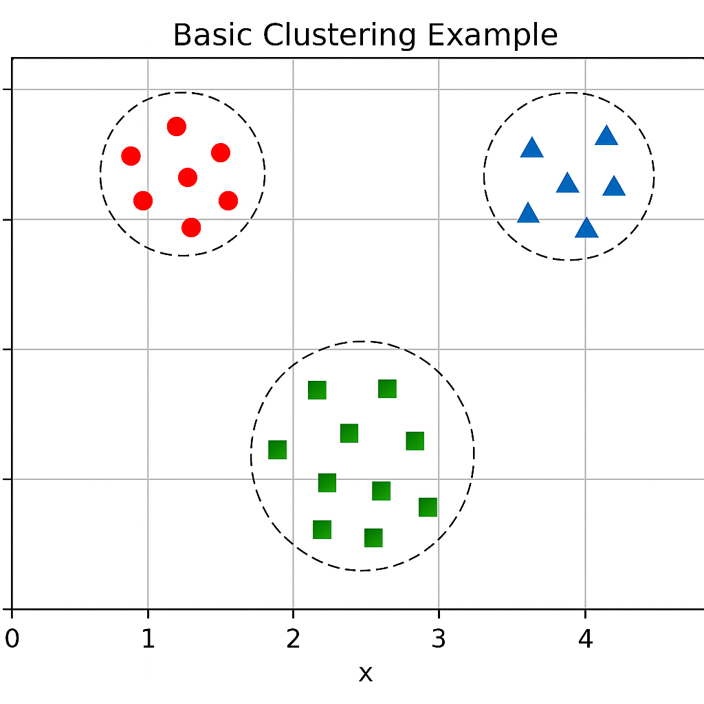
Basic Clustering Example: An illustration of how data points are grouped into distinct clusters based on their proximity.
Key Concepts and Terminology
Let's break down the essential terms you'll encounter when working with clustering. Think of these as the building blocks that help us understand and measure how well our clustering is working.
Cluster
What it is: A group of data points that are similar to each other and different from points in other groups.
Real-world analogy: Like a friend group where everyone shares similar interests, hobbies, or backgrounds.
Mathematically: A subset of your dataset where points inside are close together, and points outside are farther away.
Centroid
What it is: The "average" or center point of a cluster - like the center of gravity.
Real-world analogy: The average height and weight of all players on a basketball team represents the "typical" player.
Mathematical formula: μᵢ = (1/|Cᵢ|) Σ_{x∈Cᵢ} x (the mean of all points in the cluster)
Why it matters: Helps us understand where each cluster is "located" in our data space.
Intra-cluster Distance
What it is: How far apart points are within the same cluster.
Real-world analogy: How spread out the houses are in your neighborhood - closer houses mean a tighter neighborhood.
Good clustering: Lower intra-cluster distances mean points in the same group are very similar.
Why it matters: Tells us how "tight" or "cohesive" our clusters are.
Inter-cluster Distance
What it is: How far apart different clusters are from each other.
Real-world analogy: The distance between different neighborhoods - farther apart means clearer boundaries.
Good clustering: Higher inter-cluster distances mean clear separation between groups.
Why it matters: Tells us how well-separated our clusters are from each other.
Putting It All Together
Think of clustering like organizing a library:
- Clusters = Different sections (Fiction, Non-fiction, Science, etc.)
- Centroids = The most representative book in each section
- Intra-cluster distance = How similar books are within each section
- Inter-cluster distance = How different the sections are from each other
A well-organized library has books that are very similar within each section (low intra-cluster distance) and very different between sections (high inter-cluster distance).
The Clustering Objective
Think of clustering like organizing a perfect dinner party:
- Intra-cluster similarity (tighter groups): You want people at each table to have lots in common - maybe one table for sports fans, another for book lovers, another for music enthusiasts. The more similar people are at each table, the better the conversations will be.
- Inter-cluster dissimilarity (clear separation): You want the tables to be very different from each other. Having a table of sports fans and another table of sports fans doesn't make sense - that should be one big table. But having sports fans, book lovers, and music enthusiasts as separate tables creates distinct, interesting groups.
The fundamental goal of clustering is to maximize intra-cluster similarity while maximizing inter-cluster dissimilarity. This can be formalized mathematically as an optimization problem:
In Simple Terms:
- Intra-cluster similarity: Points within the same cluster should be as similar as possible (minimize distance between them)
- Inter-cluster dissimilarity: Different clusters should be as distinct as possible (maximize distance between clusters)
Real-world example: When Netflix recommends movies, they want to group movies that are very similar (same genre, similar ratings) and keep different types of movies in separate groups (action vs romance vs comedy).
Measuring How Good Our Clustering Is
How do we know if our clustering is good? We need a way to measure it! Think of it like grading a test - we need a scoring system.
WCSS (Within-Cluster Sum of Squares) is like a "clustering score" that tells us how well we've grouped our data. Lower scores mean better clustering!
Optimization Objective: Minimize WCSS
We want to minimize the within-cluster sum of squares (WCSS):
Formula Breakdown (Step by Step):
- WCSS: Our "clustering score" - the lower this number, the better our clustering
- Σᵢ₌₁ᵏ: "For each cluster" - we're going to check every cluster we created
- Σ_{x∈Cᵢ}: "For each point in that cluster" - we're checking every data point
- ||x - μᵢ||²: "How far is this point from the center of its cluster?" - we square this distance
- μᵢ: The center (centroid) of cluster i
In Plain English: "Add up all the distances from each point to the center of its cluster, then add up all those totals for all clusters. Lower total = better clustering!"
Real-World Analogy
Imagine you're organizing students into study groups:
- You want students with similar abilities in the same group
- WCSS measures how "spread out" students are within their groups
- Lower WCSS = students in each group are very similar to each other
- Higher WCSS = students in groups are very different from each other
Goal: Minimize WCSS to create tight, cohesive study groups!
Why is Clustering Challenging?
Clustering might sound simple, but it's actually one of the most challenging problems in machine learning. Here's why:
- No "Correct" Answer: Unlike supervised learning where we have the right answers (like "this email is spam"), clustering has no correct answer. It's like asking "What's the best way to organize a library?" - different people might have different valid opinions!
- Subjectivity of "Similarity": What makes two things "similar"? Two movies might be similar because they're both action films, or because they both have the same director, or because they're both from the 1990s. The definition depends on what you care about.
- The Curse of Dimensionality: When you have lots of features (like 100 different movie characteristics), distance calculations become meaningless. It's like trying to measure distances in a 100-dimensional space - everything seems equally far from everything else!
- Computational Complexity: Some clustering algorithms need to check every possible way to group data, which becomes impossibly slow with large datasets. It's like trying to find the best seating arrangement for 1000 people - there are too many possibilities to check them all.
- Choosing the Right Number of Groups: How many clusters should you create? Too few and you're lumping different things together. Too many and you're splitting things that should stay together. It's like deciding how many categories your store should have.
Real-world example: Imagine organizing a music streaming service. Should you group songs by genre, mood, decade, artist, or tempo? Each choice gives different results, and there's no "correct" answer - it depends on what your users want!
Understanding Unsupervised Learning
Think of machine learning like learning to cook:
- Supervised Learning: Like having a cooking teacher who shows you exactly what each dish should look like when it's done. You learn by comparing your results to the "correct" answers.
- Unsupervised Learning: Like exploring a kitchen without a teacher, discovering patterns and relationships on your own. You might notice that certain ingredients work well together, or that some cooking methods produce similar results.
To fully appreciate clustering, we must understand its place within the broader context of machine learning. Clustering belongs to the category of unsupervised learning, which fundamentally differs from supervised learning in both methodology and objectives.
The Two Main Types of Machine Learning
Imagine you're learning to identify animals:
- Supervised Learning: Someone shows you pictures with labels - "This is a cat," "This is a dog," "This is a bird." You learn by seeing examples with the correct answers.
- Unsupervised Learning: You're given a pile of animal pictures without any labels. You notice patterns on your own - maybe you group them by size, color, number of legs, or habitat, without anyone telling you the "right" way to group them.
Supervised vs Unsupervised Learning
Let's compare these two approaches side by side:
| Aspect | Supervised Learning | Unsupervised Learning |
|---|---|---|
| Data Structure | Labeled data: (X, y) pairs Like: "Email content" + "Spam/Not Spam" |
Unlabeled data: X only Like: "Email content" (no labels) |
| Objective | Learn mapping f: X → y Predict the right answer |
Discover hidden patterns in X Find interesting structures |
| Evaluation | Compare predictions with true labels "How often am I right?" |
Internal validation metrics "Do the patterns make sense?" |
| Examples | Classification, Regression Spam detection, price prediction |
Clustering, Dimensionality Reduction Customer segments, data compression |
| Mathematical Goal | Minimize prediction error Get the right answer |
Maximize data structure discovery Find meaningful patterns |
Real-World Examples
Supervised Learning:
- Email Spam Filter: Learn from labeled emails (spam/not spam)
- House Price Prediction: Learn from houses with known prices
- Medical Diagnosis: Learn from patients with known conditions
- Face Recognition: Learn from photos with labeled names
Unsupervised Learning:
- Customer Segmentation: Group customers without knowing their "type"
- Gene Expression Analysis: Find patterns in genetic data
- Market Basket Analysis: Discover which products are bought together
- Anomaly Detection: Find unusual patterns in network traffic
Visualization: Learning Paradigms Comparison
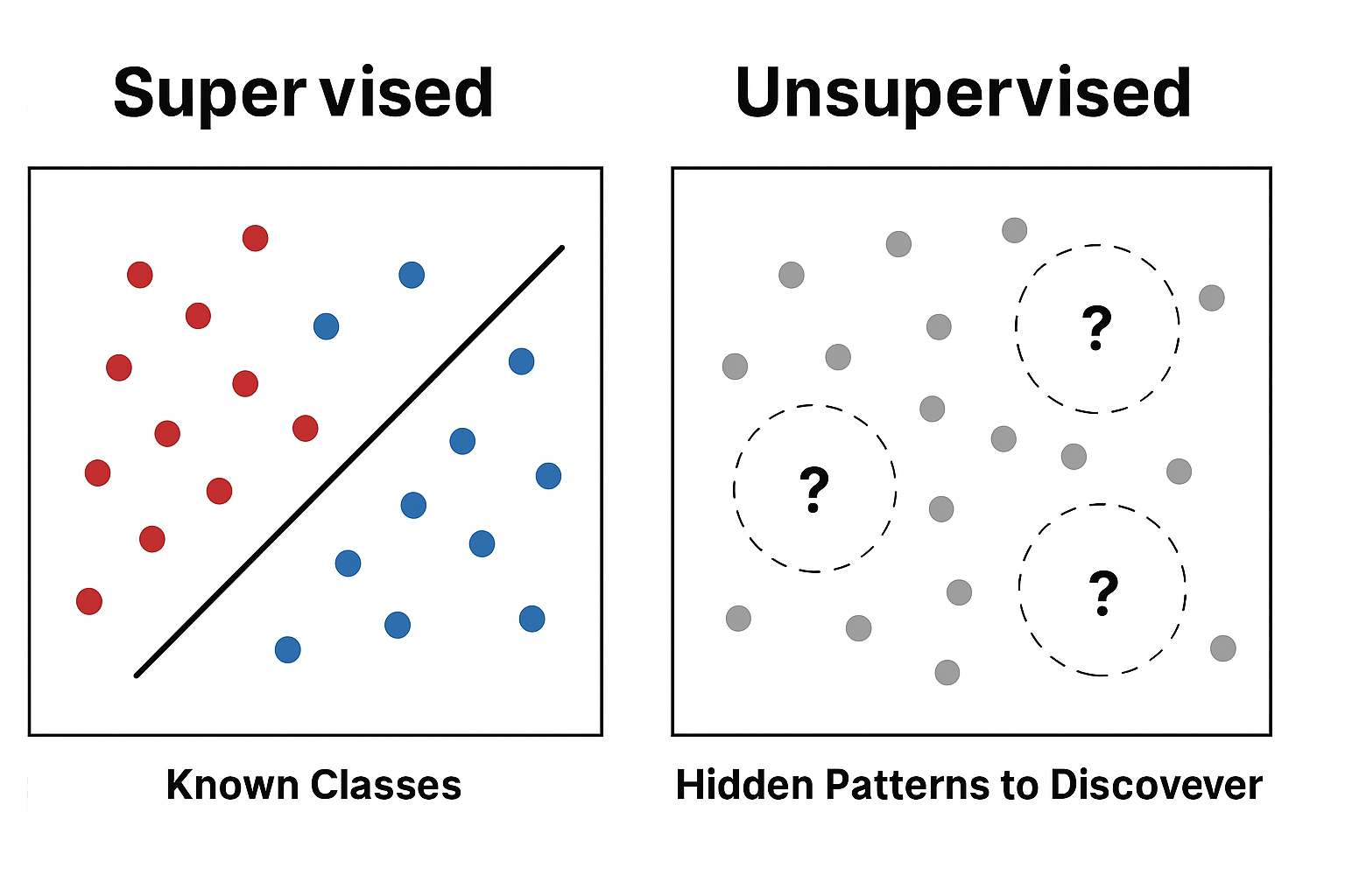
Side-by-side Comparison: See how the same dataset is approached differently in supervised learning (with labels) versus unsupervised learning (clustering without labels).
The Mathematical Framework of Unsupervised Learning
Think of unsupervised learning like being a detective with no clues:
- You have a bunch of evidence (data points) but no witness statements (labels)
- Your job is to look for patterns, connections, and groupings in the evidence
- You need to figure out what's important and what's not, all on your own
In unsupervised learning, we work with a dataset D = {x₁, x₂, ..., xₙ} where each xᵢ ∈ ℝᵈ is a d-dimensional feature vector. Our goal is to discover hidden structures, patterns, or relationships within this data without any external guidance.
In Simple Terms:
- D = Your complete dataset (like all the songs in your music library)
- x₁, x₂, ..., xₙ = Individual data points (like each individual song)
- d-dimensional = Each song has multiple features (genre, tempo, year, artist, etc.)
- Goal = Find patterns without anyone telling you what to look for
Unsupervised Learning Objectives
Common mathematical objectives in unsupervised learning include:
- Density Estimation: Estimate p(x) - the probability density function of the data
- Dimensionality Reduction: Find a lower-dimensional representation: f: ℝᵈ → ℝᵏ where k < d
- Clustering: Partition data into meaningful groups
- Association Rule Learning: Discover relationships between variables
Types of Unsupervised Learning
Unsupervised learning has several different approaches, each with its own specialty:
Clustering
What it does: Groups similar data points together
Real-world example: Organizing customers into segments like "budget shoppers," "luxury buyers," "frequent purchasers"
Algorithms: K-means, Hierarchical, DBSCAN
Output: Cluster assignments (which group each point belongs to)
Dimensionality Reduction
What it does: Simplifies complex data by reducing the number of features
Real-world example: Taking 1000 different movie characteristics and reducing them to just "action level" and "romance level"
Algorithms: PCA, t-SNE, UMAP
Output: Lower-dimensional representation (simplified data)
Anomaly Detection
What it does: Finds unusual or suspicious data points
Real-world example: Detecting fraudulent credit card transactions or equipment malfunctions
Algorithms: Isolation Forest, LOF
Output: Anomaly scores (how unusual each point is)
Association Rules
What it does: Discovers patterns and relationships between items
Real-world example: "People who buy diapers also often buy baby formula" (market basket analysis)
Algorithms: Apriori, FP-Growth
Output: Rule sets (if-then patterns)
Neural Networks
What it does: Learns representations and can generate new data
Real-world example: Creating realistic-looking fake images or learning compressed representations of photos
Algorithms: Autoencoders, VAEs, GANs, SOMs
Output: Learned features & generated samples
Density Estimation
What it does: Models how data is distributed across different regions
Real-world example: Understanding where crimes are most likely to occur in a city
Algorithms: KDE, Gaussian Mixtures, Parzen Windows
Output: Probability density functions (where data is concentrated)
Why This Matters for Clustering
Clustering is just one tool in the unsupervised learning toolbox:
- Sometimes you need clustering: When you want to group similar items together
- Sometimes you need dimensionality reduction: When your data has too many features to work with
- Sometimes you need anomaly detection: When you're looking for unusual cases
- Sometimes you combine them: First reduce dimensions, then cluster the simplified data
Understanding these different approaches helps you choose the right tool for your specific problem!
Types of Clustering Methods
Think of clustering algorithms like different tools in a toolbox:
- Different problems need different tools: You wouldn't use a hammer to cut wood, or a saw to drive nails
- Each tool has strengths and weaknesses: Some work better with certain types of data
- Understanding your options helps you choose the right one: The best algorithm depends on what you're trying to accomplish
Clustering algorithms can be categorized into several distinct types, each with its own mathematical foundations, assumptions, and optimal use cases. Understanding these categories is crucial for selecting the appropriate algorithm for your specific problem.
How to Choose the Right Clustering Method
Before diving into specific algorithms, here are the key questions to ask:
- What shape are your clusters? Round? Oval? Irregular shapes?
- Do you know how many clusters you want? Some algorithms need this number, others find it automatically
- Are there outliers or noise in your data? Some algorithms handle this better than others
- How much data do you have? Some algorithms are faster with large datasets
- Do you want to see the clustering process? Some algorithms show you step-by-step how clusters form
Partitional Clustering
Think of partitional clustering like dividing a pizza into slices:
- You decide how many slices (clusters) you want beforehand
- Each piece of pepperoni (data point) goes on exactly one slice
- You try to make the slices as even and logical as possible
- The algorithm keeps adjusting until it finds the best way to divide everything
Partitional clustering methods divide the dataset into k non-overlapping clusters. The most famous example is K-means clustering.
Characteristics of Partitional Clustering:
- Fixed Number of Clusters: You must decide how many clusters you want before starting (like deciding how many slices to cut your pizza into)
- Non-overlapping: Each data point belongs to exactly one cluster (no pepperoni can be on two slices at once)
- Optimization-based: The algorithm tries to find the best possible way to group your data (like trying different ways to cut the pizza until it looks perfect)
- Fast and Efficient: Generally works well with large datasets and is computationally efficient
When to Use Partitional Clustering:
- You know how many groups you want: Like organizing students into exactly 4 study groups
- Your clusters are roughly round: Like grouping customers by location or grouping products by category
- You have a large dataset: Partitional methods are usually faster than other approaches
- You want quick results: These algorithms typically converge quickly
Visualization: Partitional Clustering Example
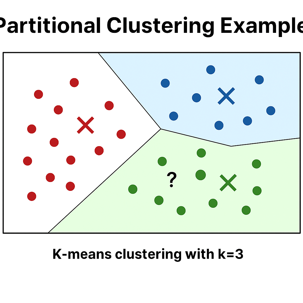
Partitional Clustering Example: A 2D plot showing K-means clustering with k=3. Data points are colored according to their cluster assignment (red, blue, green). Three large X marks indicate cluster centroids. Voronoi diagram boundaries show the decision regions for each cluster. Points clearly belong to one cluster each with no overlap.
Hierarchical Clustering
Think of hierarchical clustering like building a family tree:
- You start with individual people (data points)
- You group them into families (small clusters)
- Then group families into extended families (larger clusters)
- Finally, you might group extended families into ethnic groups (even larger clusters)
- At each level, you can see how things are related to each other
Hierarchical clustering creates a tree-like structure of clusters, representing nested groupings at different levels of granularity.
Agglomerative (Bottom-up)
How it works: Start with each point as its own cluster, then merge closest clusters iteratively
Real-world analogy: Like merging small companies into larger corporations - start with individual businesses and keep combining the most similar ones
Step-by-step process:
- Start with each data point as its own cluster
- Find the two closest clusters
- Merge them into one cluster
- Repeat until you have just one big cluster
- Choose where to "cut" the tree to get your final clusters
Divisive (Top-down)
How it works: Start with all points in one cluster, then recursively split clusters
Real-world analogy: Like breaking down a large organization into departments, then teams, then individuals - start big and keep splitting
Step-by-step process:
- Start with all data points in one big cluster
- Find the best way to split this cluster into two
- Continue splitting clusters until you reach individual points
- Choose where to stop splitting to get your final clusters
When to Use Hierarchical Clustering:
- You don't know how many clusters you want: You can explore different numbers by cutting the tree at different levels
- You want to see the clustering process: The dendrogram shows exactly how clusters were formed
- You have relatively small datasets: These methods can be slow with very large datasets
- You want to understand relationships: The tree structure shows how different groups are related
Visualization: Dendrogram Example
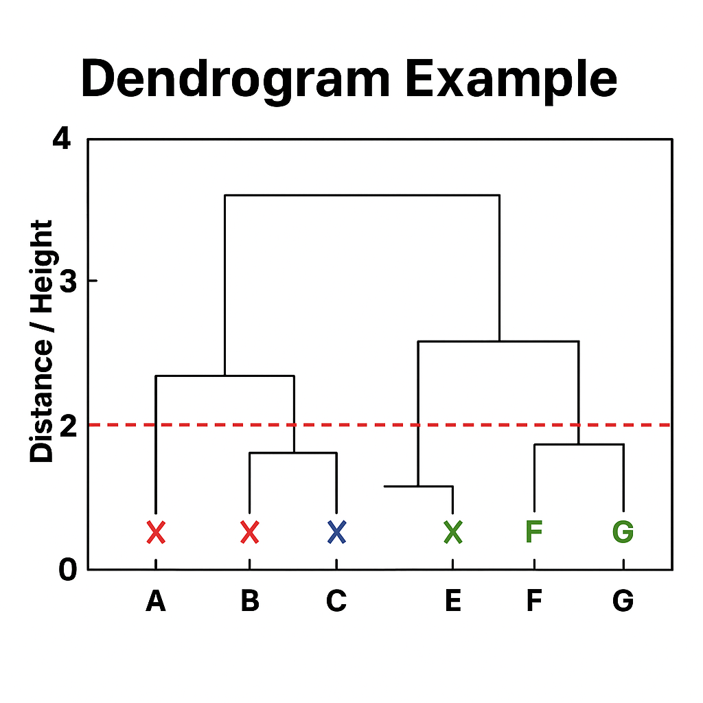
Dendrogram Example: A hierarchical tree diagram (dendrogram) showing the merging process of 8 data points labeled A through H. The y-axis shows distance/height from 0 to 4. Branches merge at different heights indicating when clusters were combined. Three main clusters are visible when cut at height 2.5, shown with a red dashed horizontal line.
Density-Based Clustering
Think of density-based clustering like finding neighborhoods in a city:
- Dense areas: Parts of the city with lots of people, buildings, and activity (these become clusters)
- Sparse areas: Empty spaces, parks, or highways that separate neighborhoods
- Arbitrary shapes: Neighborhoods don't have to be round - they can be long and thin, L-shaped, or any other shape
- Noise handling: Isolated buildings or people who don't belong to any neighborhood are identified as outliers
Density-based methods identify clusters as areas of high density separated by areas of low density. They can discover clusters of arbitrary shape and automatically handle noise.
Key Concepts in Simple Terms:
- ε-neighborhood: "Everyone within walking distance" - all points within a certain radius
- Core point: "A popular hangout spot" - a place where enough people gather to form the center of a neighborhood
- Density-reachable: "Connected by a chain of popular spots" - you can get from one point to another by following a path through popular locations
- Density-connected: "Part of the same neighborhood network" - two points that are both connected to the same central hub
Mathematical Foundation of Density-Based Clustering
For those who want the technical details:
- ε-neighborhood: Nₑ(x) = {y ∈ D | dist(x,y) ≤ ε}
- Core point: A point x where |Nₑ(x)| ≥ minPts
- Density-reachable: Point y is density-reachable from x if there exists a chain of core points connecting them
- Density-connected: Points x and y are density-connected if both are density-reachable from some point z
When to Use Density-Based Clustering:
- Your clusters have unusual shapes: Like crescent moons, spirals, or L-shapes
- You have noise or outliers: The algorithm can identify and separate these automatically
- You don't know how many clusters to expect: It finds clusters automatically based on density
- Clusters have very different sizes: Some might be much larger or smaller than others
Visualization: DBSCAN Clustering Example
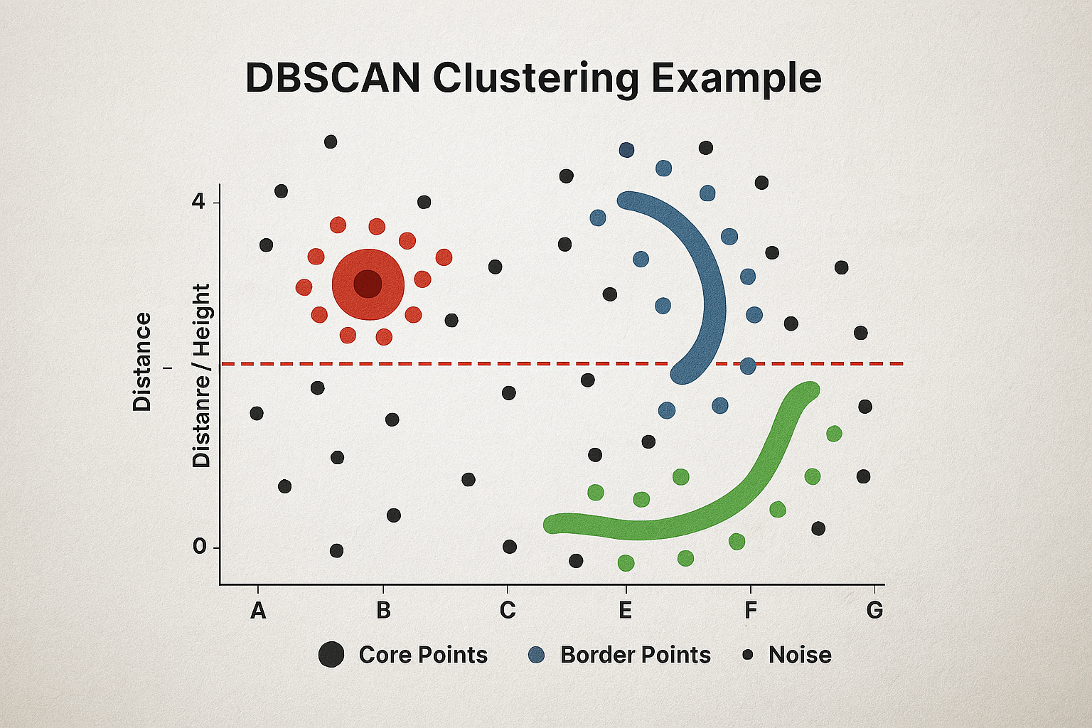
DBSCAN Clustering Example: A 2D scatter plot showing DBSCAN results with irregularly shaped clusters. Three distinct regions: (1) dense circular cluster in red, (2) crescent-shaped cluster in blue, (3) elongated cluster in green. Black dots represent noise points. Larger dots indicate core points, medium dots are border points, small dots are noise.
Model-Based Clustering
Think of model-based clustering like analyzing different recipes:
- Each cluster is like a recipe: It has specific ingredients (parameters) that define its characteristics
- Data points are like dishes: Each dish might be a mix of different recipes, but some recipes are more likely than others
- The algorithm learns the recipes: It figures out what ingredients (parameters) make each cluster unique
- Soft assignments: A dish might be 70% Italian recipe and 30% French recipe, rather than being 100% one or the other
Model-based clustering assumes that data is generated from a mixture of probability distributions. The most common approach is Gaussian Mixture Models (GMM).
What Makes Model-Based Clustering Different:
- Probabilistic approach: Instead of hard assignments (point belongs to cluster A or B), it gives probabilities (point is 80% likely to be in cluster A, 20% likely to be in cluster B)
- Learns cluster shapes: Each cluster can have its own shape, size, and orientation (not just round circles)
- Handles uncertainty: Points that are between clusters get assigned probabilities to multiple clusters
- Statistical foundation: Based on solid mathematical principles from probability theory
Gaussian Mixture Model Mathematics
A GMM represents the data as a mixture of k Gaussian distributions:
Formula Breakdown (In Plain English):
- p(x): "What's the probability of seeing this data point?"
- Σᵢ₌₁ᵏ: "Add up contributions from all k clusters"
- πᵢ: "How common is cluster i?" (like how often Italian recipes appear vs French recipes)
- 𝒩(x | μᵢ, Σᵢ): "How well does this data point fit cluster i?" (like how well a dish matches the Italian recipe)
- μᵢ: The center of cluster i (like the typical ingredients in an Italian recipe)
- Σᵢ: The shape and spread of cluster i (like how much variation is allowed in the Italian recipe)
Real-world analogy: Imagine you're trying to identify recipes from a mixed collection of dishes. Each dish has some probability of being Italian, French, Chinese, etc., based on how well it matches the typical characteristics of each cuisine.
When to Use Model-Based Clustering:
- You want soft assignments: When points might belong to multiple clusters with different probabilities
- Your clusters have different shapes: Some might be round, others oval, others stretched in different directions
- You need uncertainty estimates: You want to know how confident the algorithm is about each assignment
- You have overlapping clusters: When clusters might partially overlap in some regions
Quick Comparison: Which Method Should You Use?
Here's a quick guide to help you choose the right clustering method:
| Method | Cluster Shape | Number of Clusters | Handles Noise | Best For |
|---|---|---|---|---|
| K-means | Round/Spherical Like organizing students into study groups |
You decide beforehand Like "I want exactly 4 groups" |
No Outliers can mess it up |
Large datasets, fast results, round clusters |
| Hierarchical | Any shape Like organizing a family tree |
You choose after seeing options Like "I'll cut the tree here" |
Limited Some noise tolerance |
Small datasets, want to see clustering process |
| DBSCAN | Any shape Like finding neighborhoods in a city |
Found automatically Like "I found 3 neighborhoods" |
Yes Great at ignoring outliers |
Irregular shapes, lots of noise, unknown cluster count |
| GMM | Elliptical/Oval Like organizing recipes by cuisine |
You decide beforehand Like "I want 5 cuisine types" |
Limited Some noise tolerance |
Overlapping clusters, need probabilities, different cluster sizes |
Decision Tree: Which Algorithm Should I Use?
- Do you know how many clusters you want?
- Yes: Go to question 2
- No: Use DBSCAN or Hierarchical clustering
- What shape are your clusters?
- Round/Spherical: Use K-means
- Oval/Elliptical: Use GMM
- Irregular/Any shape: Use DBSCAN
- Do you have lots of noise/outliers?
- Yes: Use DBSCAN
- No: Any method will work
- How much data do you have?
- Large dataset (>10,000 points): Use K-means or DBSCAN
- Small dataset (<1,000 points): Any method will work
Real-World Applications
Clustering isn't just an academic exercise - it's used everywhere in the real world! From the moment you wake up and check your phone to the products you buy online, clustering algorithms are working behind the scenes to make your life better.
Clustering algorithms have found applications across virtually every domain where data analysis is performed. Understanding these applications helps contextualize the theoretical concepts and demonstrates the practical importance of clustering techniques.
Why Clustering Matters in Real Life
Think of clustering as the "organizing principle" of the digital world:
- It helps businesses understand their customers: Instead of treating all customers the same, clustering helps identify different types of customers and serve them better
- It makes technology more personal: Your phone, computer, and apps use clustering to learn your preferences and suggest things you'll like
- It helps solve complex problems: From medical research to city planning, clustering helps experts find patterns in data that humans might miss
- It saves time and money: By automatically organizing and categorizing information, clustering reduces the need for manual work
Customer Segmentation and Marketing
Imagine you own a clothing store with 10,000 customers:
- Without clustering: You send the same email to everyone - "20% off everything!" Some customers love it, others ignore it, and you waste money on irrelevant promotions.
- With clustering: You discover that your customers fall into 4 groups: "Budget-conscious families," "Luxury fashion lovers," "Trendy young adults," and "Professional business people." Now you can send targeted messages like "Family bundle deals" to families and "New designer arrivals" to luxury shoppers.
One of the most commercially successful applications of clustering is in customer segmentation, where businesses group customers based on purchasing behavior, demographics, and preferences.
Real-World Example: How Netflix Uses Clustering
Netflix doesn't just have "action movies" and "romance movies" - they have thousands of micro-genres:
- "Critically-acclaimed emotional independent films"
- "Quirky romantic comedies with strong female leads"
- "Mind-bending sci-fi thrillers"
- "Feel-good family dramas set in small towns"
They use clustering to group movies and shows based on thousands of factors: actors, directors, themes, visual style, pacing, dialogue complexity, and more. This is why their recommendations are so accurate - they're not just guessing, they're using data science!
Mathematical Approach to Customer Segmentation
Given customer data matrix X ∈ ℝⁿˣᵈ where:
- n = number of customers (like 10,000 customers)
- d = number of features (age, income, purchase frequency, favorite categories, etc.)
- xᵢⱼ = j-th feature value for customer i (like customer #1's age is 34)
The goal is to partition customers into k segments such that customers within each segment have similar purchasing patterns and can be targeted with tailored marketing strategies.
In Simple Terms: Take all the information you have about your customers (age, income, what they buy, when they buy, how much they spend) and automatically group them into similar types. Then create different marketing strategies for each group.
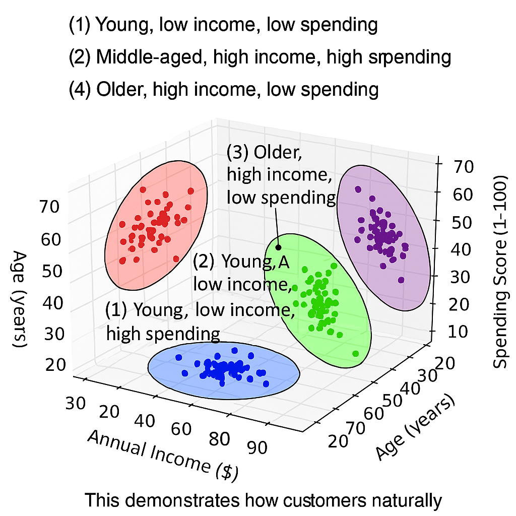
📊 Customer Segmentation Visualization
This visualization would show:
- Scatter plot of customers with different colors for each segment
- Customer segments like "Budget-conscious families," "Luxury shoppers," "Trendy young adults"
- Features like age, income, purchase frequency on the axes
- Clear separation between different customer groups
Bioinformatics and Genomics
Imagine you're a biologist trying to understand how thousands of genes work together:
- Without clustering: You'd have to manually examine each of the 20,000+ human genes individually - an impossible task!
- With clustering: You can automatically group genes that behave similarly, discovering that genes involved in "cell division" all turn on and off together, or that "immune response" genes share similar patterns.
In bioinformatics, clustering is used to analyze gene expression data, protein sequences, and other biological data to understand relationships and functions.
Real-World Example: Cancer Research
How clustering helps fight cancer:
- Gene Expression Profiling: Scientists analyze which genes are active in cancer cells vs normal cells
- Patient Stratification: Group patients with similar genetic profiles to predict treatment response
- Drug Discovery: Identify groups of proteins that work together, leading to targeted therapies
- Personalized Medicine: Match treatments to patients based on their genetic clustering profile
This has led to breakthrough treatments like Herceptin for HER2-positive breast cancer, where clustering identified a specific genetic subtype that responds to targeted therapy.
Gene Expression Analysis
What it does: Groups genes that turn on/off together
Real-world example: Discovering that 50 genes involved in "DNA repair" all activate when cells are damaged by radiation
Why it matters: Genes that work together often have similar functions - like finding all the parts of a machine that work together
Medical impact: Helps identify new drug targets and understand disease mechanisms
Protein Structure Analysis
What it does: Groups proteins by their 3D shape and structure
Real-world example: Discovering that proteins with similar shapes often have similar functions, even if they're from different species
Why it matters: Structure determines function - like how all hammers work similarly regardless of the material they're made from
Medical impact: Helps design new drugs by understanding how proteins fold and interact
Image Segmentation and Computer Vision
Think of image segmentation like organizing a messy art supply box:
- Without clustering: You have thousands of mixed-up colored pencils, markers, and crayons all jumbled together
- With clustering: You automatically group similar items - all the red pencils together, all the blue markers together, all the crayons in one section
- In images: Each pixel is like a colored pencil, and clustering groups similar pixels into objects (sky, trees, buildings, people)
Clustering plays a crucial role in computer vision for tasks like image segmentation, object recognition, and feature extraction.
Real-World Example: Medical Imaging
How clustering helps doctors see better:
- MRI Scans: Automatically separate brain tissue from tumors, blood vessels, and healthy areas
- X-rays: Identify different types of tissue (bone, muscle, lung) for better diagnosis
- Retinal Scans: Detect early signs of diabetes or glaucoma by clustering different parts of the eye
- Surgery Planning: Help surgeons identify exactly where to cut by clearly separating different anatomical structures
This technology has improved diagnosis accuracy and reduced surgery time, potentially saving lives.
Mathematical Framework for Image Segmentation
In image segmentation, we treat each pixel as a data point in a feature space:
In Simple Terms:
- R, G, B: How red, green, and blue the pixel is (like describing the color of a paint)
- X, Y: Where the pixel is located in the image (like giving an address)
- Goal: Group pixels that are both similar in color AND close together in location
Real-world analogy: It's like organizing a photo by both color and location - putting all the sky pixels together (blue and at the top), all the grass pixels together (green and at the bottom).
🖼️ Image Segmentation Process
This visualization would show:
- Original image (e.g., a landscape with sky, trees, buildings)
- Segmented result with different colors for each region
- Clear boundaries separating sky, vegetation, structures
- How pixels are grouped by color and spatial proximity
Social Network Analysis
Think of social networks like organizing a huge party:
- Without clustering: You have 1000 guests but no idea who knows whom or who should be seated together
- With clustering: You automatically discover that people naturally form groups - the "book club" group, the "sports team" group, the "work colleagues" group
- Real-world impact: This helps social media platforms suggest friends, organize content, and understand how information spreads
In social networks, clustering helps identify communities, influence groups, and patterns of interaction.
Real-World Example: Facebook's Friend Suggestions
How Facebook uses clustering to suggest friends:
- Mutual Friends Analysis: If you and someone else have many mutual friends, you're likely in the same social circle
- Activity Patterns: People who comment on similar posts or join similar groups are clustered together
- Location-Based Clustering: People from the same school, workplace, or neighborhood form natural clusters
- Interest-Based Groups: People who like similar pages, attend similar events, or share similar content
This clustering helps Facebook create a more connected and engaging social experience.
Graph-Based Clustering Mathematics
Given a graph G = (V, E) representing a social network:
- V = set of users/nodes (like all the people at the party)
- E = set of connections/edges (like who knows whom)
- Adjacency Matrix A: Aᵢⱼ = 1 if edge exists between users i and j (like a guest list showing who knows whom)
In Simple Terms: Community detection algorithms find groups where people know lots of others in their group but few people outside their group - like natural friend circles at a party.
Financial Services and Fraud Detection
Think of fraud detection like being a security guard at a mall:
- Normal shoppers: Follow predictable patterns - enter through main doors, browse stores, make purchases, leave
- Suspicious behavior: Someone who enters through the back, goes straight to expensive items, tries to leave quickly without paying
- Clustering helps: Automatically identify normal shopping patterns and flag anything that doesn't fit
Real-World Example: Credit Card Fraud Prevention
How banks use clustering to protect your money:
- Transaction Clustering: Your normal spending patterns (coffee shops, gas stations, grocery stores) form a "normal" cluster
- Anomaly Detection: When a transaction appears that doesn't fit your cluster (like buying expensive jewelry in another country), it gets flagged
- Real-time Protection: The system can freeze suspicious transactions before they complete, protecting your account
- Learning from Patterns: The system continuously learns from new transactions, updating your "normal" cluster over time
This technology has prevented billions of dollars in fraudulent transactions and saved countless people from financial loss.
Credit Card Fraud Detection
What it does: Identifies unusual spending patterns that might indicate fraud
Real-world example: Flagging a $2000 purchase at a jewelry store in Paris when you normally only buy coffee and groceries in your hometown
How it works: Creates clusters of "normal" transactions for each user, then identifies transactions that don't fit any cluster
Impact: Prevents billions in fraudulent transactions annually
Portfolio Management
What it does: Groups stocks with similar risk and return characteristics
Real-world example: Discovering that tech stocks, healthcare stocks, and energy stocks each form distinct clusters with different risk profiles
How it works: Analyzes historical performance, volatility, and correlation to group similar investments
Impact: Helps investors build diversified portfolios and manage risk
Healthcare and Medical Diagnosis
Think of medical clustering like organizing patients in a hospital:
- Without clustering: Every patient gets the same treatment, regardless of their specific condition or response to medications
- With clustering: Patients with similar symptoms, genetic profiles, or treatment responses are grouped together for personalized care
- Real-world impact: This leads to more effective treatments, fewer side effects, and better patient outcomes
Medical applications of clustering range from patient stratification to drug discovery and epidemiological studies.
Real-World Example: Cancer Treatment Personalization
How clustering revolutionizes cancer treatment:
- Genetic Profiling: Cluster patients based on their genetic mutations to predict which treatments will work best
- Response Prediction: Group patients who respond similarly to chemotherapy to optimize treatment plans
- Side Effect Management: Identify patients likely to experience similar side effects for proactive care
- Drug Development: Group patients with similar disease characteristics for more targeted clinical trials
This personalized approach has improved survival rates and quality of life for cancer patients worldwide.
🏥 Patient Clustering for Personalized Medicine
This visualization would show:
- Patient data points grouped by genetic profiles
- Different clusters representing treatment-responsive groups
- Features like gene expression levels, biomarkers
- How patients with similar profiles respond to treatments
Document Classification and Text Mining
Think of text clustering like organizing a huge library:
- Without clustering: You have millions of documents but no way to organize them - like having every book in the world piled in one giant heap
- With clustering: Documents automatically get sorted into topics - all the cooking books together, all the history books together, all the science fiction together
- Real-world impact: This helps search engines, news aggregators, and content platforms organize and recommend relevant content
In natural language processing, clustering helps organize documents, identify topics, and analyze sentiment patterns.
Real-World Example: News Organization
How Google News uses clustering to organize articles:
- Topic Clustering: Automatically groups articles about the same news story from different sources
- Sentiment Analysis: Clusters articles by positive, negative, or neutral sentiment about the same topic
- Source Diversity: Ensures you see multiple perspectives on the same story by clustering by content similarity
- Trend Detection: Identifies emerging topics by clustering similar new articles
This helps readers get comprehensive coverage of important news stories from multiple angles.
Text Clustering Mathematics
Documents are typically represented using the Vector Space Model:
- TF-IDF Vector: xᵢⱼ = tfᵢⱼ × log(N/dfⱼ)
- tfᵢⱼ: Term frequency of word j in document i (how often the word appears in this document)
- dfⱼ: Document frequency of word j (how many documents contain this word)
- N: Total number of documents
In Simple Terms: TF-IDF gives higher weight to words that are common in a specific document but rare across all documents - like how "pizza" gets high weight in a cooking article but low weight in a sports article.
Challenges and Assumptions
Think of clustering like being a detective:
- You have evidence (data) but no witnesses (labels): You need to figure out what's important and what's not
- Every detective has different methods: Some are better at finding certain types of clues
- Some cases are easier than others: Clear evidence makes the job easier, messy evidence makes it harder
- You need to know the limitations: Understanding what can go wrong helps you avoid mistakes
While clustering is a powerful tool for data analysis, it comes with significant challenges and limitations that must be understood to apply these techniques effectively. These challenges stem from both theoretical limitations and practical implementation issues.
Why Understanding Challenges Matters
Knowing the challenges helps you:
- Choose the right algorithm: Like picking the right tool for the job
- Interpret results correctly: Understanding when to trust your results and when to be skeptical
- Avoid common mistakes: Like using the wrong algorithm for your data type
- Set realistic expectations: Knowing what clustering can and cannot do
The Fundamental Challenge: Defining Similarity
Think of defining similarity like organizing a music collection:
- By Genre: Rock, Jazz, Classical - but where does "Alternative Rock" fit?
- By Mood: Happy, Sad, Energetic - but what about "melancholy but uplifting"?
- By Era: 80s, 90s, 2000s - but what about artists who span decades?
- By Instrument: Guitar-heavy, Piano-based - but what about orchestral pieces?
All of these are valid ways to group music, but they produce completely different clusters! The same data can be clustered in many different meaningful ways.
The core challenge in clustering is that the notion of "similarity" is inherently subjective and context-dependent. What constitutes a meaningful cluster varies dramatically across domains and applications.
Real-World Example: Customer Segmentation
The same customers can be grouped in multiple valid ways:
- By Demographics: Age groups, income levels, geographic regions
- By Behavior: Frequent buyers, occasional shoppers, bargain hunters
- By Preferences: Brand loyalists, variety seekers, quality-focused
- By Life Stage: Students, young professionals, families, retirees
Each grouping reveals different insights and supports different business strategies. There's no single "correct" way to cluster customers!
Multiple valid clusterings can exist for the same dataset
The Curse of Dimensionality
Think of the curse of dimensionality like trying to find someone in a huge city:
- In a small town: "Find the person with brown hair" - there might be 10 people, easy to find!
- In a medium city: "Find the person with brown hair and blue eyes" - still manageable with more details
- In a huge metropolis: "Find the person with brown hair, blue eyes, 5'8", wearing red shirt, size 10 shoes, born in March..." - now everyone starts to look the same because there are so many combinations!
With too many features (dimensions), every data point becomes equally "different" from every other point, making clustering nearly impossible.
As the number of features increases, distance-based clustering algorithms face fundamental mathematical challenges that can render them ineffective.
Real-World Example: Online Shopping
Imagine trying to recommend products based on customer preferences:
- With 2 features (age, income): Easy to group customers - young professionals, families, retirees
- With 10 features: Still manageable - add location, education, hobbies, etc.
- With 1000 features: Every customer becomes unique - their browsing history, purchase patterns, device types, time of day preferences, color preferences, brand loyalty scores, price sensitivity, review patterns, social media activity, and 990 other features!
This is why companies use dimensionality reduction techniques before clustering - to focus on the most important features.
Mathematical Analysis of High-Dimensional Distance
In high-dimensional spaces, the ratio of the maximum to minimum distance approaches 1:
This phenomenon, known as the "concentration of distances," means that all points appear equidistant in high-dimensional spaces, making clustering based on distance metrics ineffective.
Consequences for Clustering:
- Distance metrics lose discriminative power
- Nearest neighbor relationships become less meaningful
- Cluster boundaries become less distinct
- Traditional algorithms may fail to find meaningful clusters
The Parameter Selection Problem
Most clustering algorithms require the specification of parameters that significantly affect the results, yet there's often no principled way to choose these parameters.
K-means: Number of Clusters (k)
Challenge: How to choose k?
Methods: Elbow method, silhouette analysis, gap statistic
Limitation: No universally optimal approach
DBSCAN: ε and minPts
Challenge: Sensitive to parameter choices
Methods: k-distance plots, domain knowledge
Limitation: Different densities require different parameters
Hierarchical: Linkage and Cut Height
Challenge: Which level to cut the dendrogram?
Methods: Gap statistics, stability analysis
Limitation: Single linkage vs complete linkage trade-offs
Computational Complexity Challenges
Many clustering algorithms have high computational complexity, making them impractical for large datasets.
Complexity Analysis of Common Algorithms
| Algorithm | Time Complexity | Space Complexity | Scalability |
|---|---|---|---|
| K-means | O(nkt) | O(n + k) | Good |
| Agglomerative HC | O(n³) | O(n²) | Poor |
| DBSCAN | O(n log n) | O(n) | Moderate |
| Spectral Clustering | O(n³) | O(n²) | Poor |
Where: n = number of data points, k = number of clusters, t = number of iterations
The Evaluation Problem
Unlike supervised learning, clustering lacks ground truth labels, making evaluation subjective and challenging.
Types of Clustering Validation
- Internal Validation: Based only on the data and clustering results
- Silhouette coefficient
- Calinski-Harabasz index
- Davies-Bouldin index
- External Validation: Compares results to known ground truth
- Adjusted Rand Index
- Normalized Mutual Information
- Fowlkes-Mallows Index
- Relative Validation: Compares different clustering algorithms
- Stability analysis
- Cross-validation approaches
- Consensus clustering
Initialization and Local Optima
Many clustering algorithms are sensitive to initialization and can get trapped in local optima, leading to inconsistent results.

How initialization affects final clustering results
Assumptions of Common Clustering Algorithms
Each clustering algorithm makes implicit assumptions about the data structure. Violating these assumptions can lead to poor results.
K-means Assumptions
- Clusters are spherical (isotropic)
- Clusters have similar sizes
- Clusters have similar densities
- Features are continuous and scaled
- No outliers in the data
Hierarchical Clustering Assumptions
- Nested cluster structure exists
- Distance metric is meaningful
- Linkage criterion matches data structure
- No noise points
- Computational resources are sufficient
DBSCAN Assumptions
- Clusters have uniform density
- Clusters are separated by low-density regions
- Parameter ε is appropriate for all clusters
- Distance metric captures similarity well
- Noise points can be identified
Strategies for Addressing Clustering Challenges
Best Practices for Robust Clustering
- Data Preprocessing:
- Feature scaling and normalization
- Dimensionality reduction for high-dimensional data
- Outlier detection and treatment
- Algorithm Selection:
- Understand data characteristics and assumptions
- Try multiple algorithms and compare results
- Use ensemble clustering methods
- Parameter Tuning:
- Use systematic parameter selection methods
- Apply cross-validation when possible
- Incorporate domain knowledge
- Validation:
- Use multiple evaluation metrics
- Perform stability analysis
- Validate results with domain experts
Mathematical Foundations
Think of mathematical foundations like learning the rules of a game:
- You don't need to be a math expert: Just like you don't need to be a professional athlete to enjoy playing basketball
- Understanding the basics helps you play better: Knowing the rules helps you understand why certain strategies work
- We'll explain everything step-by-step: Like learning to drive - we'll go through each concept one at a time
- Real-world analogies make it easier: We'll use everyday examples to explain mathematical concepts
Understanding the mathematical foundations of clustering is essential for selecting appropriate algorithms and interpreting results correctly.
Why Mathematical Understanding Matters
Understanding the math helps you:
- Choose the right algorithm: Know which mathematical approach fits your data
- Troubleshoot problems: Understand why an algorithm isn't working as expected
- Optimize performance: Know which parameters to adjust for better results
- Interpret results correctly: Understand what the numbers actually mean
Distance Metrics
Think of distance metrics like different ways to measure how far apart two cities are:
- Straight-line distance: Like measuring "as the crow flies" - shortest path
- Driving distance: Following actual roads and highways - more realistic for travel
- Travel time: How long it actually takes to get there - accounts for traffic, road conditions
- Cost of travel: How much it costs to get there - includes gas, tolls, etc.
Each method gives you a different "distance" between the same two cities, and each is useful for different purposes!
Euclidean Distance
The most commonly used distance metric in clustering:
Formula Breakdown (In Plain English):
- d(x, y): The distance between point x and point y
- √: Take the square root (like finding the hypotenuse of a triangle)
- Σᵢ₌₁ᵈ: "Add up for each feature" - go through each dimension
- (xᵢ - yᵢ)²: "Square the difference" - like (3-1)² = 4
Real-world analogy: Like measuring the straight-line distance between two points on a map - the shortest possible distance.
When to Use:
- Continuous numerical data (like height, weight, temperature)
- Features are on similar scales (all in meters, all in dollars, etc.)
- Spherical clusters expected (like organizing students by height and weight)
When NOT to Use:
- Categorical data (like "red", "blue", "green" - you can't subtract colors!)
- Features on very different scales (height in meters vs income in thousands of dollars)
- High-dimensional data (too many features make distances meaningless)
Manhattan Distance
Also known as L1 norm or city block distance:
Formula Breakdown (In Plain English):
- d(x, y): The distance between point x and point y
- Σᵢ₌₁ᵈ: "Add up for each feature" - go through each dimension
- |xᵢ - yᵢ|: "Absolute difference" - like |3-1| = 2 (always positive)
Real-world analogy: Like walking through Manhattan - you can only go up/down and left/right on the city blocks, never diagonally across buildings. It's the sum of horizontal and vertical distances.
When to Use:
- High-dimensional data (works better than Euclidean with many features)
- Outliers are present (less sensitive to extreme values)
- Features have different scales (more robust to scale differences)
- City-like navigation (GPS routing, robot pathfinding)
Real-World Example:
Taxi navigation in Manhattan: A taxi can't drive through buildings, so it must follow the street grid. The Manhattan distance gives the actual driving distance, while Euclidean distance would be the "as the crow flies" distance.
Cosine Similarity
Measures the angle between vectors, ignoring magnitude:
When to Use:
- Text data and document clustering
- High-dimensional sparse data
- When magnitude is less important than direction
Evaluation Metrics
Silhouette Coefficient
The silhouette coefficient is one of the most intuitive and widely-used clustering evaluation metrics. It measures how similar an object is to its own cluster compared to other clusters, providing a clear indication of clustering quality.
Formula Breakdown:
- a(i): Average distance from point i to all other points in the same cluster (intra-cluster distance)
- b(i): Average distance from point i to all points in the nearest neighboring cluster (inter-cluster distance)
- s(i): Silhouette coefficient for point i
- Range: [-1, 1] where 1 = well-clustered, 0 = on cluster boundary, -1 = misclassified
How to Use Silhouette Coefficient:
- Calculate for each point: Compute s(i) for every data point in your dataset
- Average across all points: Take the mean of all silhouette coefficients to get the overall score
- Interpret the results:
- 0.7 - 1.0: Strong clustering structure
- 0.5 - 0.7: Reasonable clustering structure
- 0.25 - 0.5: Weak clustering structure
- < 0.25: No substantial clustering structure
When to Use Silhouette Coefficient:
- Cluster validation: When you need to validate the quality of your clustering results
- Optimal k selection: To find the best number of clusters by comparing silhouette scores for different k values
- Algorithm comparison: To compare different clustering algorithms on the same dataset
- Outlier detection: Points with negative silhouette coefficients might be outliers or misclassified
Calinski-Harabasz Index (Variance Ratio Criterion)
The Calinski-Harabasz Index, also known as the Variance Ratio Criterion, is a statistical measure that evaluates clustering quality by comparing the ratio of between-cluster variance to within-cluster variance. It's particularly useful for partitional clustering algorithms like K-means.
Formula Breakdown:
- SSB (Sum of Squares Between): Total squared distance between cluster centroids and the overall centroid
- SSW (Sum of Squares Within): Total squared distance between data points and their cluster centroids
- k: Number of clusters
- n: Number of data points
- (k-1): Degrees of freedom for between-cluster variance
- (n-k): Degrees of freedom for within-cluster variance
Higher values indicate better clustering - more separation between clusters and tighter clusters
How to Use Calinski-Harabasz Index:
- Calculate for different k values: Compute CH index for various numbers of clusters
- Find the maximum: The k value with the highest CH index is typically optimal
- Compare algorithms: Use CH index to compare different clustering algorithms
- Statistical significance: Higher CH values indicate statistically significant cluster separation
When to Use Calinski-Harabasz Index:
- K-means optimization: Particularly effective for finding optimal k in K-means clustering
- Spherical clusters: Works best when clusters are roughly spherical and similar in size
- Large datasets: Computationally efficient for large datasets
- Algorithm comparison: Good for comparing partitional clustering algorithms
Davies-Bouldin Index
The Davies-Bouldin Index is a clustering evaluation metric that measures the average similarity ratio of each cluster with its most similar cluster. Unlike other metrics, lower values indicate better clustering quality, making it intuitive to interpret.
Formula Breakdown:
- Sᵢ: Average distance from points in cluster i to cluster i's centroid (intra-cluster scatter)
- Sⱼ: Average distance from points in cluster j to cluster j's centroid (intra-cluster scatter)
- Mᵢⱼ: Distance between centroids of clusters i and j (inter-cluster separation)
- max_{j≠i}: Maximum value over all clusters j different from i
- Σᵢ₌₁ᵏ: Sum over all k clusters
- (1/k): Average over all clusters
Lower values indicate better clustering - tighter clusters with better separation
How to Use Davies-Bouldin Index:
- Calculate for each cluster: Compute the ratio (Sᵢ + Sⱼ) / Mᵢⱼ for each cluster i with its most similar cluster j
- Find the maximum ratio: For each cluster, find the maximum ratio across all other clusters
- Average the results: Take the average of all maximum ratios to get the final DB index
- Interpret the score: Lower values (closer to 0) indicate better clustering
When to Use Davies-Bouldin Index:
- Cluster validation: When you need a simple, interpretable measure of clustering quality
- Optimal k selection: To find the best number of clusters by minimizing the DB index
- Algorithm comparison: To compare different clustering algorithms on the same dataset
- Compact clusters: Particularly effective when you expect compact, well-separated clusters
Vector Spaces and Data Representation
All clustering algorithms operate on data represented as vectors in a mathematical space. Understanding this representation is crucial for algorithmic success.
Mathematical Data Representation
Given a dataset D with n observations and d features:
Where each observation xᵢ ∈ ℝᵈ is a d-dimensional vector:
The choice of feature space ℝᵈ and the scaling of features significantly impacts clustering results.
Optimization Theory in Clustering
Most clustering algorithms can be formulated as optimization problems. Understanding these formulations helps in algorithm design and analysis.
K-means as an Optimization Problem
K-means Objective Function
K-means minimizes the within-cluster sum of squared errors (WCSS):
Where:
- k = number of clusters
- Cᵢ = set of points in cluster i
- μᵢ = centroid of cluster i
Lagrangian Formulation:
The optimal centroid for each cluster is the mean of points in that cluster:
This can be proven by taking the derivative of J with respect to μᵢ and setting it to zero.
Gradient Descent in Clustering
Some clustering algorithms use gradient-based optimization to find optimal solutions.
Gradient Descent for Clustering
For a general clustering objective function J(θ), gradient descent updates parameters as:
Where:
- α = learning rate
- ∇J(θₜ) = gradient of objective function at iteration t
This approach is used in algorithms like Gaussian Mixture Models with EM algorithm.
Information Theory in Clustering
Information theory provides tools for measuring cluster quality and comparing clustering results.
Mutual Information
Measures the amount of information shared between two clustering assignments:
Where:
- P(i) = probability that a point belongs to cluster i in clustering C
- P'(j) = probability that a point belongs to cluster j in clustering C'
- P(i,j) = joint probability
Normalized Mutual Information (NMI):
Where H(C) is the entropy of clustering C.
Interactive Clustering Demonstration
Think of this interactive demo like a science experiment:
- You're the scientist: You get to design your own experiments and see what happens
- You control the variables: Change the data, adjust the settings, and watch the results change
- You learn by doing: See the concepts in action rather than just reading about them
- You can experiment safely: Try different combinations without any consequences
Experience clustering algorithms in action with this interactive demonstration. You can generate different datasets, adjust parameters, and see how various algorithms perform in real-time.
What You'll Learn from This Demo
By experimenting with this demo, you'll understand:
- How clustering algorithms work: See the step-by-step process in action
- Why different parameters matter: Change the number of clusters and see how it affects results
- How data affects clustering: Generate different types of data and see which algorithms work best
- Real-world applications: See how the concepts apply to actual problems
Interactive K-means Clustering Demo
This demo lets you:
- Generate your own data: Create different patterns and see how K-means handles them
- Control the algorithm: Adjust the number of clusters and see how it affects the results
- Watch step-by-step: See exactly how the algorithm finds clusters, one step at a time
- Compare distance metrics: See how different ways of measuring "distance" affect clustering
- Evaluate results: Learn how to measure whether clustering worked well
Generate random data and watch K-means algorithm find clusters step by step.
How to Use This Demo
Step-by-step guide:
- Start with "Generate New Data": This creates a random dataset for you to experiment with
- Adjust the parameters: Try different numbers of clusters and see how it changes the results
- Run the algorithm: Click "Run K-means" to see the algorithm work automatically
- Or step through manually: Use "Step Through Algorithm" to see each step one by one
- Try different distance metrics: Compare how Euclidean, Manhattan, and Cosine distances affect clustering
- Evaluate the results: Look at the metrics to see how well the clustering worked
Click "Generate New Data" to start the demonstration
Distance Metrics Comparison
Compare how different distance metrics affect clustering results on the same dataset.
Cluster Evaluation Metrics
Understand how different evaluation metrics assess clustering quality.
Visualization: Algorithm Performance Comparison
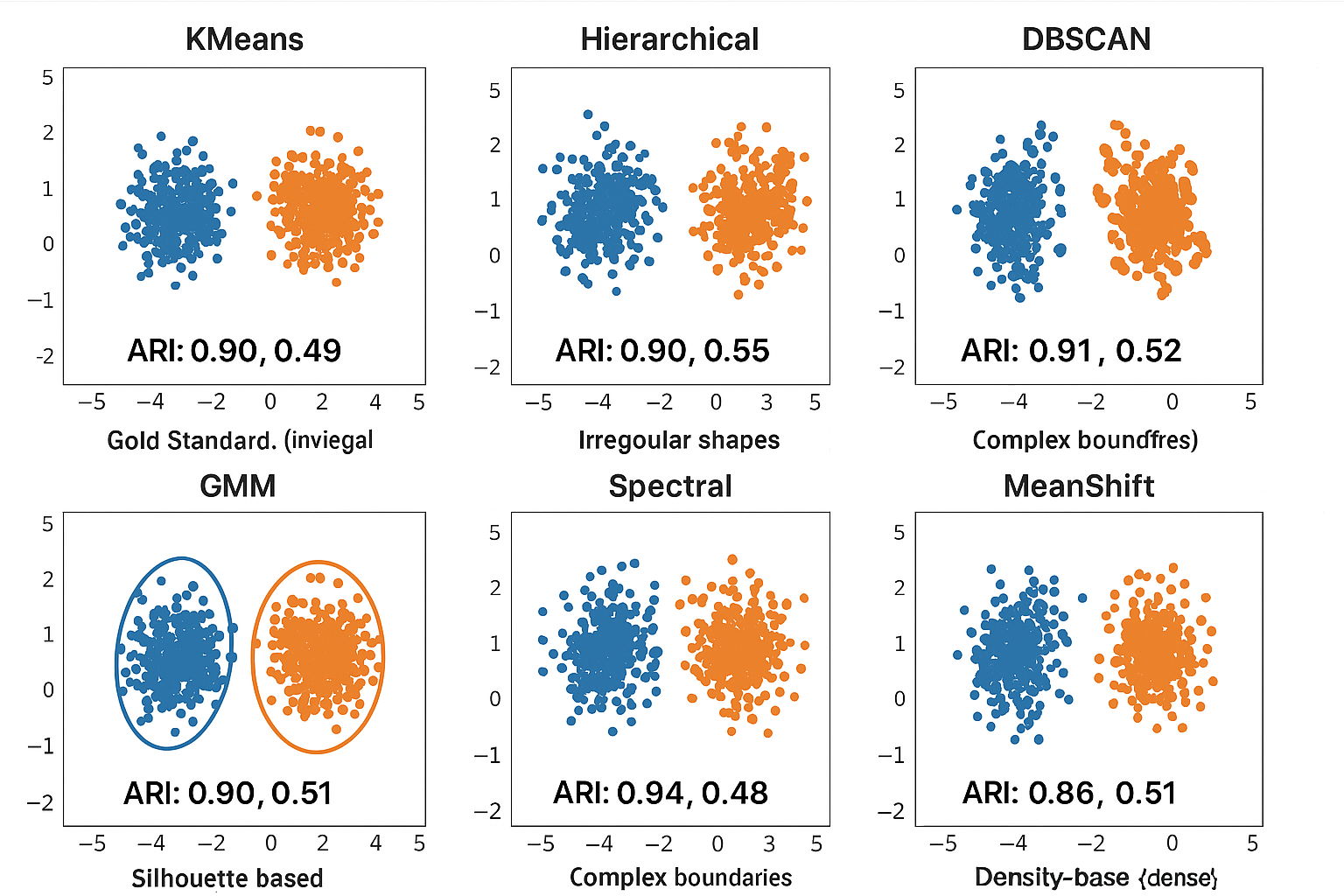
Algorithm Performance Comparison: A 2x3 grid showing the same dataset clustered by different algorithms: K-means (spherical clusters), Hierarchical (dendrogram-based), DBSCAN (irregular shapes), GMM (elliptical), Spectral (complex boundaries), and Mean Shift (density-based). Each subplot shows the algorithm name, clustering result with different colors, and evaluation metrics below.
Test Your Clustering Knowledge
Think of this quiz like a practice test:
- It's okay to get questions wrong: That's how you learn! Wrong answers help you identify what to review
- Each question teaches you something: Even if you get it right, the explanation reinforces your understanding
- It's not about the score: It's about making sure you understand the key concepts
- You can take it multiple times: Practice makes perfect!
Evaluate your understanding of clustering fundamentals, unsupervised learning concepts, and mathematical foundations.
What This Quiz Covers
This quiz tests your understanding of:
- Basic clustering concepts: What clustering is and why it's useful
- Unsupervised learning: How it differs from supervised learning
- Distance metrics: Different ways to measure similarity between data points
- Algorithm selection: When to use different clustering methods
- Real-world applications: How clustering is used in practice
Don't worry if you don't get everything right the first time - that's normal! The goal is to learn.
Question 1: Clustering Goal
What is the primary goal of clustering?
Question 2: Algorithm Types
Which of the following is NOT a type of clustering algorithm?
Question 3: WCSS Definition
What does WCSS stand for in clustering?
Quiz Score
Correct answers: 0 / 3